Using pasture information when deciding what to trade
Spring 2022 is set-up to be another productive season for graziers in Australia’s south-east. Most areas are close to maximum saturation condition for soil moisture. As temperature and daylight hours increase, conditions shortly should be ideal for optimum pasture growing conditions. It will be the management of spring growth and a likely feed surplus in most systems, that will determine whether an operation cash’s in on these conditions.
In Article 1 of this series, we looked at determining pasture quantity and quality on farm. At this time of year and under the current seasonal conditions, few producers would be concerned about future feed availability. However, maximising feed utilisation and maintaining feed quality are going to be more challenging. It is under these conditions, that increasing stocking rate through a trade enterprise we can achieve these two outcomes and increase profit for an operation.
So, what should we consider in terms of pasture budgets and trading margins for a trade operation? Let’s look at a simple scenario for a spring trade to understand these factors.
Budgeting Pasture Growth and Utilisation
We will utilise MLA’s Feedbase planning and budgeting tool, specifically the ‘How many hectares do I need?’ model to calculate pasture growth and utilisation for a breeding herd scenario. For the trade scenario we can also use this tool, but given it models livestock at maintenance condition, we will use the MLA Stocking Rate Calculator with a determined daily pasture intake as per the Data tables from Prograze, NSW DPI and MLA.
Scenario 1: Meeting the cow-herd requirements
We have a spring calving operation in a high rainfall region (>650 mm per annum) who has traditionally conserved fodder during spring and focussed on building a summer bank of feed. After successive back-to-back growing seasons, the hay shed and strategically buried silage pits are now full. They haven’t fed out supplementary feed in the past 2 years and are thinking about trade options this season, to maximise spring pasture utilisation and quality.
This operation has access to an area of 100 hectares of improved pasture with some legume content. They allocate paddocks to the herd through a combination of set-stocking and rotational grazing practices depending on the time of the year.
They are coming off a low feed level out of winter (1,200 kg DM/ha) and wish to build a sufficient volume of feed to cover summer grazing requirements (estimating 2,500 kg DM as a starting point for December).
We can model different scenarios by month or season to complete a whole farm budget. For this example, we will model spring (1st September to 30th November).
Scenario 1 Input
We will budget for average growth conditions across September to December, and on digestibility that is associated with green grass (minimal/low legume content) in an early-mid vegetative stage. We are feed budgeting for 100 cows and calves (early to mid-lactation) over this period. The cows are an average of 600 kg liveweight (LWT), which is higher than usual, as cows are at present a fat score 4. Normally they sit at a 2.5-3.0 fat score and closer to 500 kg LWT.
| Current feed on offer (FOO): | 1,200 kg DM/ha |
| Desired FOO when animals removed: | 2,500 kg DM/ha |
| Consumptive Wastage factor: | 70% dig, 10 MJ ME/kg – Green, grassy |
| Pasture Growth: | 40% |
| Number of days animals are in the paddock: | 55 kg DM/ha/dy |
| STOCK 1 | 91 |
| Stock type | Cows |
| Average weight | 600 kg/hd |
| Physiological state | Early Lactation (2 months) |
| Twins / singles / not applicable | Not applicable |
| Number of animals grazing | 100 |
| Scenario 1 output: | |
|---|---|
| Estimated pasture intake (kg DM/Hd/day) | 11.7 |
| Maintenance energy required (MJ ME/Hd/day) | 167 |
| Total pasture intake + wastage (Kg DM/ha/day) | 148,548 |
| Total growth minus change in FOO (KG DM/ha) | 3,750 |
| Total area required (hectares) | 40.1 |
The initial modelling shows we still have 59 hectares (59%) of potential grazing area and feed base still available. Let us consider two options to utilise this excess feed; trade steers and trade lamb weaners.
Scenario 2: Trade steers
It’s often these next calculations that can be more challenging to model. This is because we need to consider stocking rate and pasture availability and then determine the associated liveweight gain. We are going to model a purchase of trade steers at 400 kg LWT purchased on the 1st September and sold at 491 kg LWT on the 30th November. This equates to 91 kg LWT gain in 91 days at an average daily gain of 1.0 kilograms liveweight per head per day (kg LWT/hd/dy).
Utilising the ‘Data Tables’ associated with the MLA’s Feedbase planning and budgeting tool, we can determine cattle DM intake and performance based on the modelled scenario as per table 3.
| Cattle Liveweight (kg LWT) | Pasture intake (kg DM/hd/dy) | Average Daily Gain |
|---|---|---|
| 400 | 9.3 | 1.1 |
| 450 | 9.7 | 1.0 |
| 500 | 9.9 | 0.9 |
Scenario 2 input
We will now model an average 450 kg LWT animal and 1.0 kg/hd/dy in the MLA Stocking Rate Calculator (Beef). This assumes 9.7 kg dry matter intake per head per day (kg DM/hd/dy) with a 40% wastage factor. This equates to 14 kg DM/hd/dy (rounded up to nearest kg).
| Trade Feeder Steers | |
|---|---|
| Paddock Size | 59 |
| Pasture available at start of grazing: | 1,200 kg DM/ha |
| Pasture available at end of grazing: | 2,500 kg DM/ha |
| Pasture Quality: | 70% dig, 10 MJ ME/kg – Green, grassy |
| Consumptive Wastage factor: | 40% |
Scenario 2 Output
| Alternative Allowance (10MJ ME/kg DM) | 14 kg DM/head/day |
| Pasture Growth: | 55 kg DM/ha/dy |
| Stocking rate hd /paddock area | 171 hd / 59 ha |
We have now determined we can support an additional 171 steers at an average liveweight of 450 kg over spring.
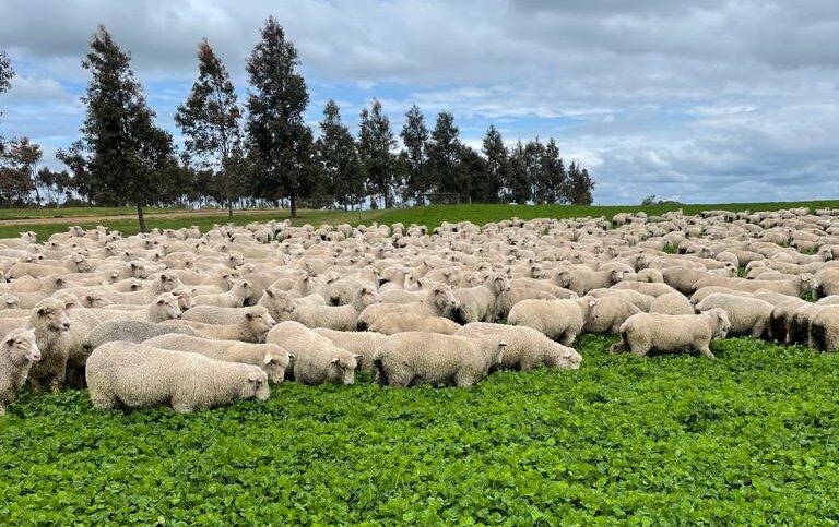
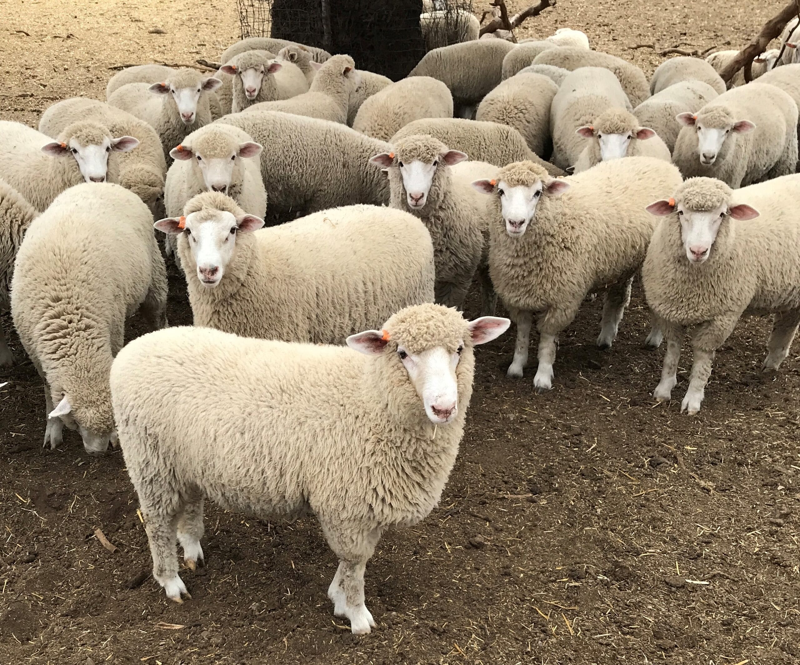
Scenario 3: Weaner lambs
As an alternative to steers, we can assess a purchase of trade lamb weaners. For this trade, purchase and sale dates will be the same as Scenario 2. Lambs will average 32.5 kg LWT (30-35 kg range on 1st September) at purchase and be sold at 48.5 kg LWT (46 – 51 kg range) on the 30th November. This equates to 16 kg LWT gain in 91 days at an average daily gain of 175 g LWT/hd/dy. Lambs will follow cattle and clean up feed residuals at 1,000 – 1,500 kg DM/ha. Utilising the same ‘Data Tables’ we can determine the pasture intake required to meet this rate of gain as per table 6.
| Lamb Liveweight (kg LWT) | Pasture intake (kg DM/hd/dy) | Average Daily Gain (g LWT/hd/dy) |
|---|---|---|
| 25 | 1.1 | 175 |
| 35 | 1.3 | 175 |
| 45 | 1.5 | 175 |
Scenario 3 Input:
We will now model an average 40.5 kg LWT lamb assuming 175 g/hd/dy in the MLA Stocking Rate Calculator (Sheep). This assumes 1.4 kg DM/hd/dy with 40% wastage factor equating to 2 kg DM/hd/dy (round to the nearest whole kg for the model).
| Trade Weaner Lambs | |
|---|---|
| Paddock Size | 59 |
| Pasture available at start of grazing: | 1,500 kg DM/ha |
| Pasture available at end of grazing: | 1,000 kg DM/ha |
| Pasture Quality: | 70% dig, 10 MJ ME/kg – Green, grassy |
| Pasture Growth: | 55 kg DM/ha/dy |
| Consumptive Wastage factor: | 40% |
Scenario 3 output:
| Alternative Allowance (10MJ ME/kg DM) | 2 kg DM/head/day |
| Stocking rate hd /paddock area | 1,687 hd / 49 ha |
We have now determined we can support an additional 1,687 lambs at an average liveweight of 40.5 kg over spring.
Which trade? Evaluating your options
To determine which is the best trading option, we will require a simple gross margin analysis. For this example, we will use the following data sources:
- The MLA National restocker lamb indicator value 02/09/22
- The MLA trade lamb indicator value 02/09/22
- The MLA feeder trade steer indicator value 02/09/22
- Aggregate Consulting’s average trade cattle and sheep enterprise expenses for 2021/22
To keep this trade evaluation simple, we will assume lambs do not require shearing or crutching. We have also converted $ per kg carcass weight ($/ kg CWT) to $/ kg LWT for lamb at a 47% dressing percentage.
| Trade Steers | Trade Lambs | |
| PURCHASE 1ST SEPT | ||
| Average Weight (kg LWT) | 400 | 32.5 |
| Average Price ($/kg LWT) | $5.01 | $3.03 |
| Average Price ($/hd) | $2,004 | $98 |
| Number of head | 171 | 1,687 |
| TOTAL TRADE PURCHASE VALUE | $342,684 | $165,952 |
| Mortality % | 2% | 2% |
| Mortalities (Number of Head) | 4 | 34 |
| SALE – 30th NOV | ||
| Average Weight (kg LWT) | 491 | 48.5 |
| Average Price ($/kg LWT) | $5.01 | $3.40 |
| Average Price ($/hd) | $2,460 | $165 |
| Number of head sold | 167 | 1653 |
| TOTAL TRADE SALE VALUE | $410,805 | $272,804 |
| NET INCOME | ||
| $ /head sold | $407.91 | $64.64 |
| TOTAL TRADE NET INCOME | $68,121 | $106,852 |
| ENTERPRISE EXPENSES $/HD | ||
| A/Health & Breeding | $26.87 | $5.70 |
| Freight | $70.69 | $7.17 |
| Insurance | $0.08 | $0.09 |
| Materials | $0.54 | $0.07 |
| Selling Costs: Stock | $100.33 | $16.50 |
| TOTAL EXPENSES $/HD SOLD | $200.86 | $29.79 |
| TOTAL TRADE EXPENSES | $33,543 | $49,247 |
| GROSS MARGIN | ||
| $ /head sold | $207.05 | $34.85 |
| TOTAL GROSS MARGIN FOR TRADE | $34,578 | $57,605 |
Based on the gross margin evaluation, weaner lambs are the best trade option, resulting in an additional $23,027 gross margin for the operation. It should be noted that the higher lamb profit is influenced by the premium of $0.37 kg/LWT in sale of finished trade lambs versus the restocker lamb purchase price. In the case of the feeder steers, there was no difference between the purchase and sale price modelled as per current market conditions.
Return On Investment & impact of market fluctuations
The final considerations for these two options are the Return On Investment (ROI) and the potential impact of market fluctuations on trading profitability. In table 10 and 11, we review the impact on variation in purchase and sales prices on the trade outcome for gross margin $ per head. Blue cells indicate a gross margin generating a ROI greater than 50%, green cells indicate an ROI between 50% and 20%, yellow cells indicate an ROI between 20% and 10%, and the red indicates an ROI below 10%.
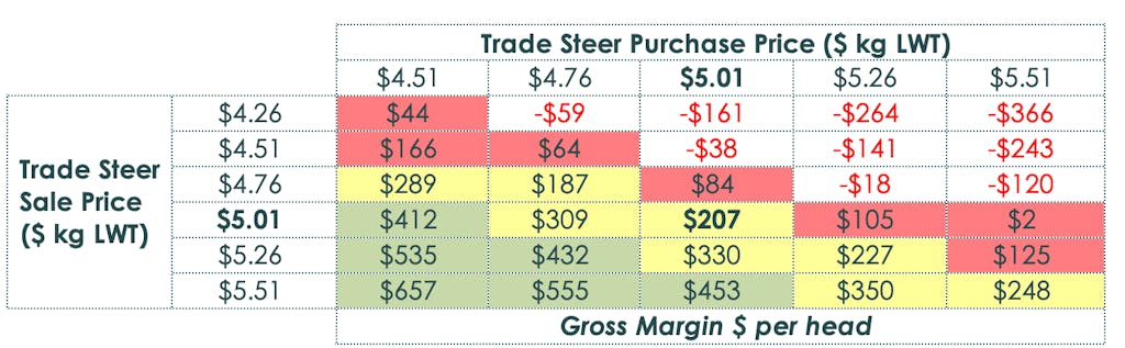
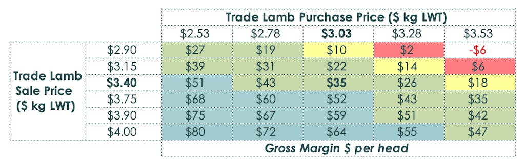
Our final assessment and overall conclusion for the scenarios modelled; the lamb trade produces the greatest gross margin ($34.85 per head) and total gross margin of $57,605 for a return-on-investment of 35%. Furthermore, the trade also results in a more favourable outcome (gross margin and ROI) under both increasing or decreasing sale price conditions.
MLA’s Feedbase planning and budgeting tool and stocking rate calculators are great tools for computing pasture growth and utilization for a variety of breeding herd scenarios. However, return on investment (ROI) and market fluctuations still have to be factored in to determine profitability.
In need of livestock financing? Talk to one of our livestock funding agents today. Agrifunder is ready to help with your funding requirements.
Author
Aggregate Consulting is an agricultural consultancy business based in Wagga Wagga in southern NSW.
Related Posts
-
![]()
Assessing pasture quantity and quality
Managing pasture quantity and quality across different seasons, are crucial aspects of optimising livestock performance. Pasture budgeting provides opportunities to both increase carry capacity or identify feed shortages in advance of the surplus or deficit.
READ MORE -
![]()
Buying and selling livestock - a guide to managing risk when trading
Livestock trading is a useful tool for boosting farm incomes when surplus feed is available. To confidently trade it is best to do the sums for a range of opportunities now, setting yourself some benchmark returns to cover the risks. That way you won’t miss opportunities for want of not being prepared.
READ MORE -
![]()
Making the most of better seasons by trading cattle
Although there is not much we can be certain about when it comes to the production and market risk in farming, there is one thing we know for sure. To generate maximum profits over the long term requires capitalising on the above average seasons.
READ MORE -
![]()
Is there still a margin in store lamb trading?
To gain some insight into how traders can assess their trading options and navigate the associated risk, Aggregate Consulting provides an overview of the fundamentals of trading livestock and a case-study on trading store lambs in the current market.
READ MORE -
![]()
Restocking in a high price beef cattle market?
Aggregate shares some insights
Many producers will have started the 2021 season with surplus feed, and together with beef prices at historically high levels, there is huge opportunity for businesses to generate unprecedented profits in the beef industry.
READ MORE -
![]()
How to source funding for livestock
Although we are operating in a dynamic and often uncertain environment, one thing is for sure – the product you produce (red meat) is essential and therefore is in demand through even the worst of events e.g. COVID-19. To keep up with this demand and ensure supply of production, funding is required – we can help you with that.
READ MORE -
![]()
How to get a livestock loan in Australia to support your business growth
We talk a lot about opportunity cost and the importance of being clear about the goals of your business when determining your business plan. This naturally flows through to how you review your finance options for livestock.
READ MORE